The ideas on this page are inspired by this Youtube video.
Here, we explore a method of visualizing of complex valued functions i.e. functions of the form $f:\mathbb C\to\mathbb C$. Specifically, we are interested in complex valued polynomials (though the same techniques could be applied to any arbitrary function).
Given a polynomial of the form
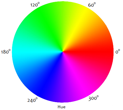
\[f(z)=a_0+a_1z+\cdots+a_dz^d\]we evaluate $f$ over the complex unit circle, that is, we compute $f(z)$ for every $z\in\mathbb C$ such that $|z|=1$. The values $f(z)$ are plotted on the complex plane and coloured based on $\arg(z)$; specifically, we map the range $[0,2\pi]$ in $\arg(z)$ to the “H” (hue) component of the HSL colour space.
As an example, the below program visualizes the polynomial
\[f(z)=z^3+iz\]Input Shape
Polynomial
Controls
- Use the scrollwheel to zoom in and out of the diagram (TODO: panning is not yet supported)
- In the “Polynomial” section, you can modify the coefficients of the polynomial $a_i$ and the degree $d$
- In the “Input Shape” section, you can adjust the radius of the circle that the function is evaluated over, and also evaluate the function over regular $n$-gons instead of circles
- Note that for reference, the input values to the function (i.e. the complex unit circle by default) have also been plotted using darker colours
A Neat Example
A neat example is to trace out
\[f(z)=-(z-1)^2=-z^2+2z-1\]over the unit circle.
This produces a unit cardioid (i.e. a cardioid with $a=1$).
Proof
Since the inputs lie on the unit circle, write $z=\cos t+i\sin t$. Then
\[\begin{align*} f(z)&=f(\cos t+i\sin t)\\ &=-(\cos t+i\sin t-1)^2\\ &=-(\cos t-1)^2+\sin^2t-2(\cos t-1)i\sin t\\ &=(-\cos^2t+2\cos t-1+\sin^2t)+(2\sin t-2\cos t\sin t)i\\ &=(1-2\cos^2t+2\cos t-1)+(2\sin t-2\cos t\sin t)i\\ &=2\cos t(1-\cos t)+2\sin t(1-\cos t)i \end{align*}\]and $(2\cos t(1-\cos t),2\sin t(1-\cos t))$ are exactly the parametric equations of a unit cardioid.
TODO: Add a geometric argument.
Fundamental Theorem of Algebra
Recall the fundamental theorem of algebra.
Fundamental Theorem of Algebra
Let $f$ be a polynomial of degree $d$ i.e.
\[f(z)=a_0+a_1z+\cdots+a_dx^d\]with $a_i\in\mathbb C$ for $0\leq i\leq d$ and $a_d\neq 0$.
Then $f$ has $d$ (complex) roots, counting multiplicity.
We can use the above visualization to argue why this should be true. The following argument is adapted from the YouTube video mentioned at the start.
Proof of the Fundamental Theorem of Algebra
Let $f(z)=a_0+a_1z+\cdots a_dx^d$ be a polynomial of degree $d$. Suppose we evaluate $f$ over a large enough circle in the complex plane. Then the behaviour of $f$ is dominated by the leading term, that is $f(z)\sim a_dz^d$, hence the output shape is approximately a circle which is much larger than the input circle. By making the input circle $z$ arbitrarily large, the output circle $a_dx^d$ grows arbitrarily large as well. Conversely, if we evaluate $f$ over a small enough circle then $f$ can be approximated by $f(z)\sim a_0+a_1z$ which is a small circle around $a_0$. Again by making the input circle $z$ arbitrary small, the output circle $a_0+a_1z$ grows arbitrary small as well, tending to just the single point $a_0$ in the limit.
Now, if $a_0=0$ then by shrinking $|z|\to 0$ we see that $f(z)\to 0$ hence $f$ has a root at $z=0$. Otherwise if $a_0\neq 0$, then somewhere between the two extremes above, there must be some intermediate circle that we evaluate $f$ over such that $f(z)=0$ for some $z$ lying on that intermediate circle.
This shows that a polynomial of degree $d$ has at least one root say $\alpha$. We can divide $f(z)$ by $z-\alpha$ to produce a new polynomial $\hat f(z)=\frac{f(z)}{z-\alpha}$ of degree $d-1$ and repeat this process until we are left with a degree 1 polynomial which clearly has one root. Hence the original polynomial $f$ of degree $d$ must have $d$ roots counting multiplicity.
Computing Roots
We can use the argument in the proof to approximately compute the roots of any polynomial. As an example, consider the polynomial
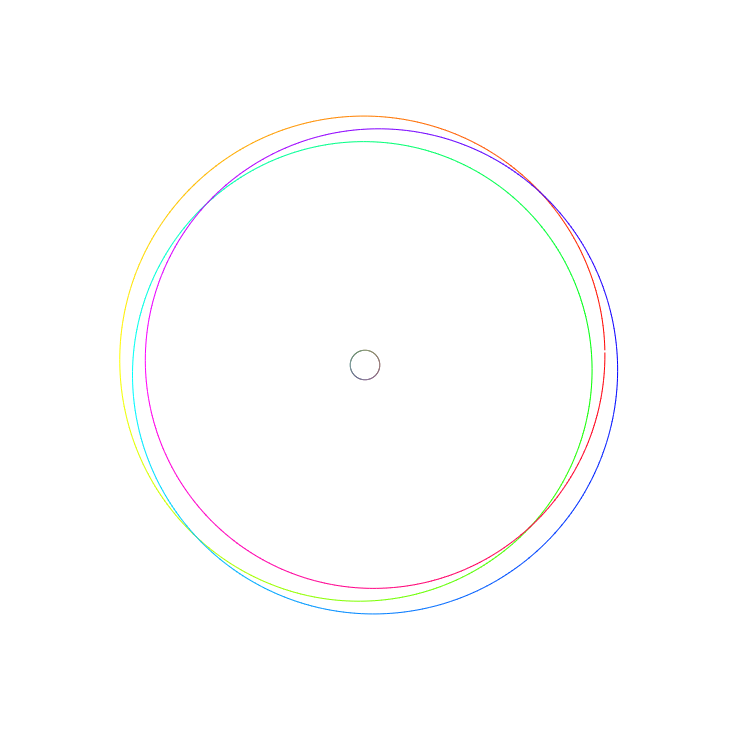
\[f(z)=z^3+iz+1.\]Shown below is its behaviour when applied over the unit circle.
$f(z)$ evaluated over the unit circle.
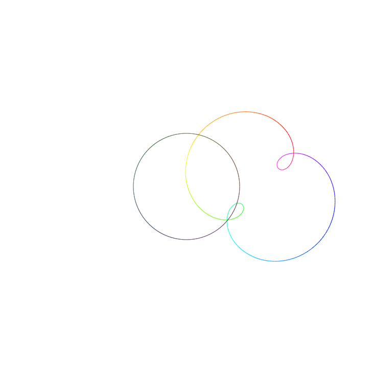
We now investigate what happens when we evaluate $f$ over a small circle and a large circle. In the two images below we use $r=0.1$ and $r=0.4$ respectively.
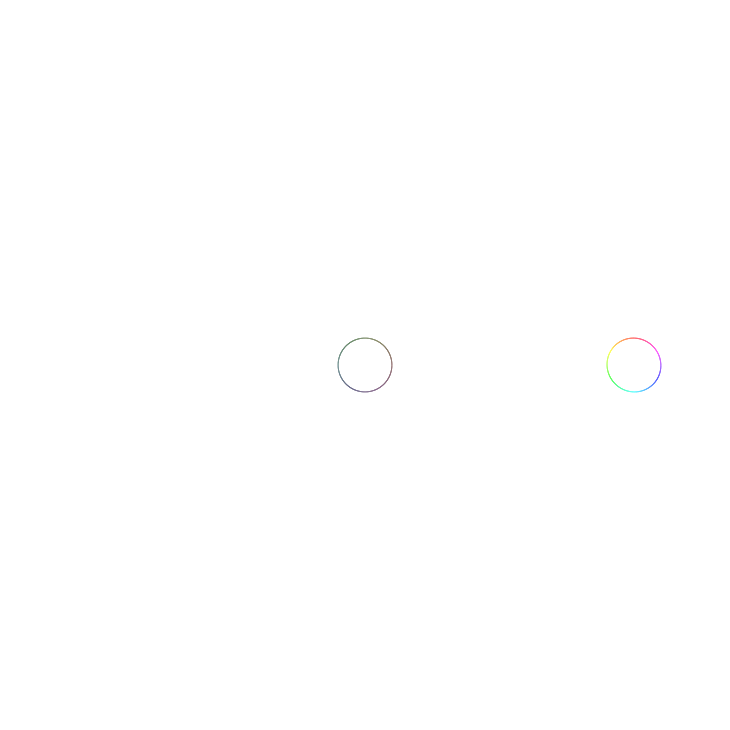
$f(z)$ evaluated over a circle with radius $r=0.1$.
$f(z)$ evaluated over a circle with radius $r=4$.
Consistent with our argument earlier, we see that when evaluating $f(z)$ over a circle with a large radius, the output is an even bigger approximate-circle, and when evaluating $f(z)$ over a circle with a small radius, the output is a small approximate-circle centered around $a_0=1$.
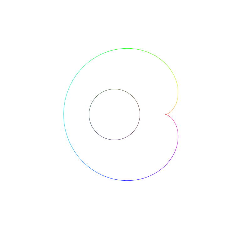
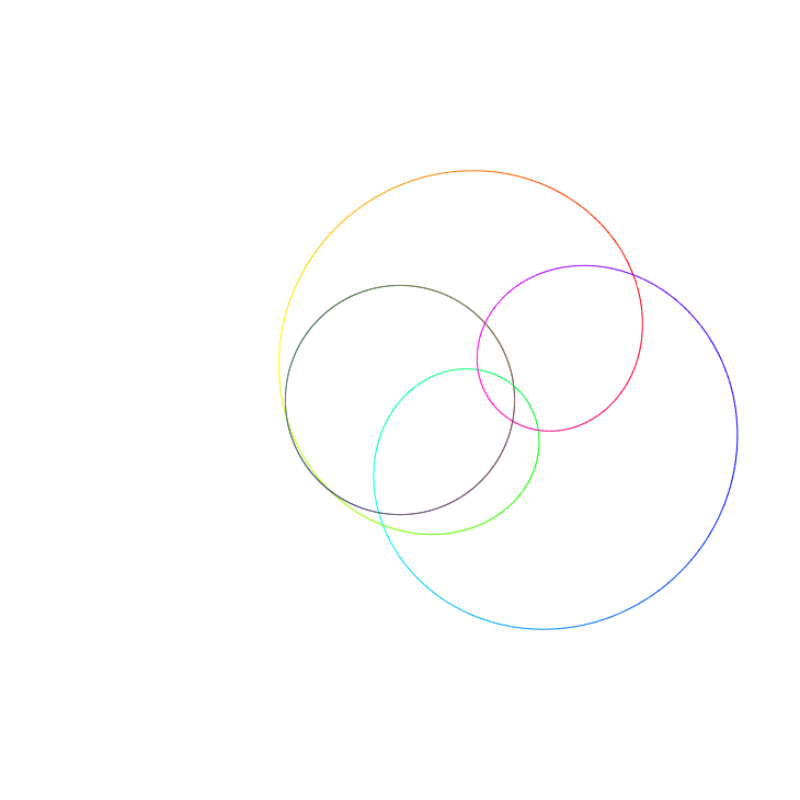
Now let’s try finding an intermediate input circle so that our polynomial $f(z)$ has a root (i.e. crosses the origin). If we start from $r=0.1$ and slowly increase the radius $r$, we’ll see that around $r=0.73$ the output crosses the origin. This tells us that one of the roots of $f$ has magnitude appropximately $0.73$. Furthermore, since the part of the output that crosses the origin is yellow in colour, we know (from this diagram) that the argument must be approximately $\frac{\pi}{3}$. Hence one of the roots is $z\approx 0.73e^{\frac{\pi}{3}i}\approx 0.73e^{1.05i}$.
$f(z)$ evaluated over a circle with radius $r=0.73$.
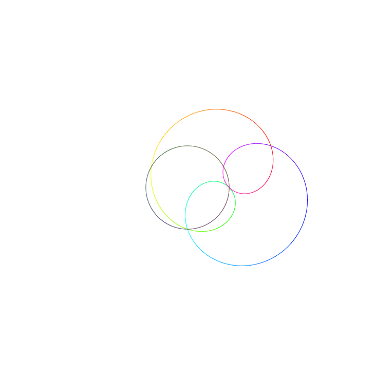
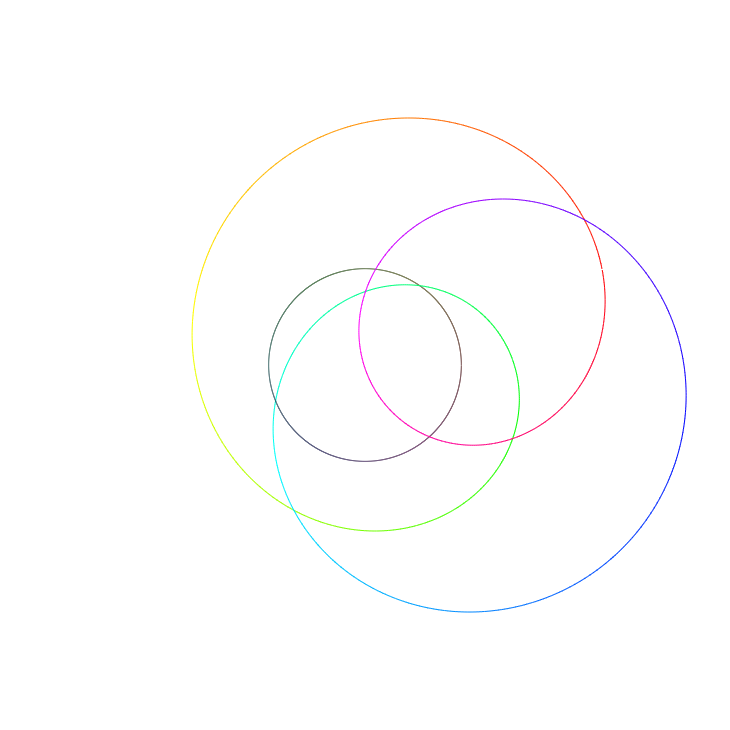
What’s more, we can even compute the two other roots (which are guaranteed to exist by the fundamental theorem). If we continue to increase $r$ we see that at around $r=1.06$ the output curve intersects with the origin once again. This time the colour is somewhere between light blue and green, corresponding to an argument of approximately $\frac{5}{6}\pi$. Hence a second root is $z\approx 1.06e^{\frac 56\pi i}\approx 1.06e^{2.62i}$.
$f(z)$ evaluated over a circle with radius $r=1.06$.
Finally, increasing $r$ again gives a third root at around $r=1.3$ which is pink in colour, corresponding to an argument of approximately $\frac 53\pi$. Hence a third root is $z\approx 1.3e^{\frac 53\pi i}=1.3e^{-\frac 13\pi i}\approx 1.3e^{-1.05i}$.
$f(z)$ evaluated over a circle with radius $r=1.3$.
If you increase $r$ further, notice that the output curve will never cross the origin again, confirming that indeed there are only three roots to this cubic polynomial.
To conclude, we’ve discovered that the three roots to the polynomial $f(z)=z^3+iz+1$ are approximately
- $z\approx 0.73e^{1.05i}$
- $z\approx 1.06e^{2.62 i}$
- $z\approx 1.3e^{-1.05 i}$.
How do our crude approximations compare with the actual roots? Mathematica tells me the roots are
- $z\approx 0.7259e^{1.2563i}$
- $z\approx 1.0624e^{2.8105i}$
- $z\approx 1.2967e^{-0.9252i}$.
Our magnitude approximations were pretty spot on; our approximations for the argument were not so great, but that’s to be expected as we estimated that by eyeballing the colours of the output curve.