There are a lot of articles, blogs, Youtube videos, etc. out there that introduce neural networks, however most of these do not discuss the mathematics behind neural network training in depth, which is what really interested me when I first learn about neural networks. Two valuable resources I found that did discuss this were Andrew Ng’s “Neural Networks and Deep Learning” course on Coursera and Michael Nielsen’s online book of the same title, both of which I highly recommend you check out if you are interested in this topic. I wanted to present here my own take on deriving the backpropagation equations for neural network training; my approach involves developing a framework for computing derivatives of matrix valued functions.
I first introduce briefly what a neural network is, so that you will be able to follow along even without any prior knowledge. I then introduce my framework for computing derivatives, and then I derive the backpropagation equations using the framework.
Introduction
We start off with a regression problem, similar to what we had for linear regression. As before, suppose we are given $m$ training example pairs $x^{(i)},y^{(i)}$ for $i=1,\cdots,m$ where $x^{(i)}\in\mathbb R^{ n},y^{(i)}\in\mathbb R$ and we want to predict $y$ from $x$. In linear regression we used a linear (technically, affine) function to predict $y$ from $x$ by making the prediction $\hat y=w^T\cdot x$. In order to simplify notation later on, we will write this instead as $\hat y=x^T\cdot w$.
Of course, if the relationship between $y$ and $x$ is non-linear, then this model will not perform very well. Let $z:=x^T\cdot w$. In order to introduce some non-linearity to our model, we introduce a non-linear activation function $g:\mathbb R\to\mathbb R$ that we apply to $z$, which gives us
\[a=g(z)=g(x^T\cdot w)\]which is called the activation value. Common choices for $g$ include the sigmoid function $g(z)=\frac{1}{1+e^{-z}}$ or the ReLU function $g(z)=\max(0,z)$.
Unlike linear regression, we will use multiple sets of weights. Call the first set of weights $w_1$ and the first activation value $a_1$ so that
\[a_1=g(x^T\cdot w_1).\]We can apply the same process with a different set of weights $w_2$ and obtain a different activation value
\[a_2=g(x^T\cdot w_2)\]and so on. Let $n^{[1]}$ denote the number of different weights we used. Then in general we compute
\[a_i=g(x^T\cdot w_i)\]for $i=1,2,\cdots,n^{[1]}$. To summarise, the setup we have currently looks like this
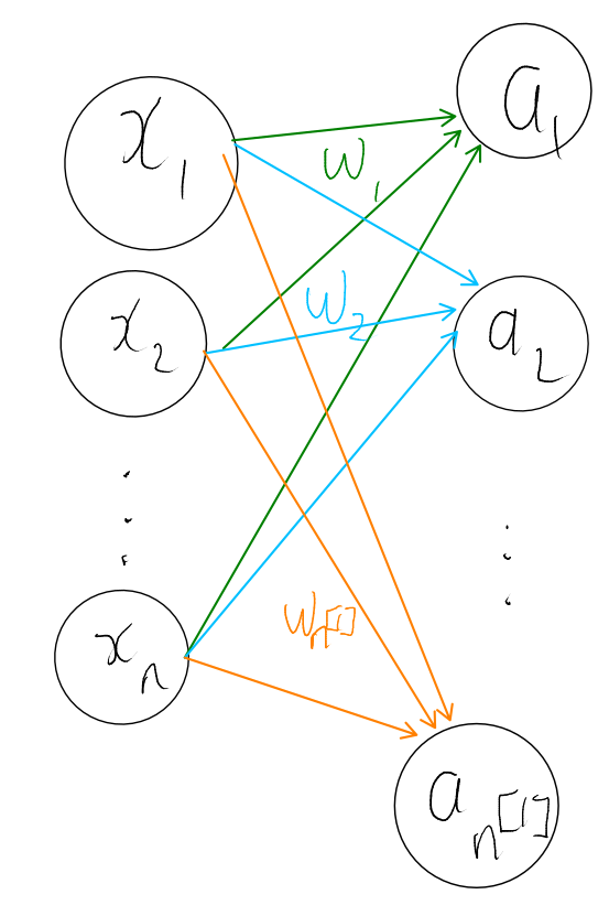
One layer neural network.
We call this a neural network with one layer. The circles or activation values are the “neurons” or nodes in the network.
We can add more layers by considering all the activation values as a vector $a^{[1]}\in\mathbb R^{n^{[1]}}$, treating it as an input, and repeating the same process. That is, we have a set of new weights, say $w^{[2]}_1,w^{[2]}_2,\cdots,w^{[2]}_{n^{[2]}}$ and we compute the activation values in the second layer as
\[a_i^{[2]}=g^{[2]}(z^{[2]}_i)\]where
\[z^{[2]}_i:=({a^{[1]}}^T\cdot w_i^{[2]}).\]The superscript of $[2]$ denotes which layer we are considering so $w^{[2]}$ are the weights of the second layer, $g^{[2]}$ is the activation function in the second layer and $a^{[2]}$ are the activation values in the second layer.
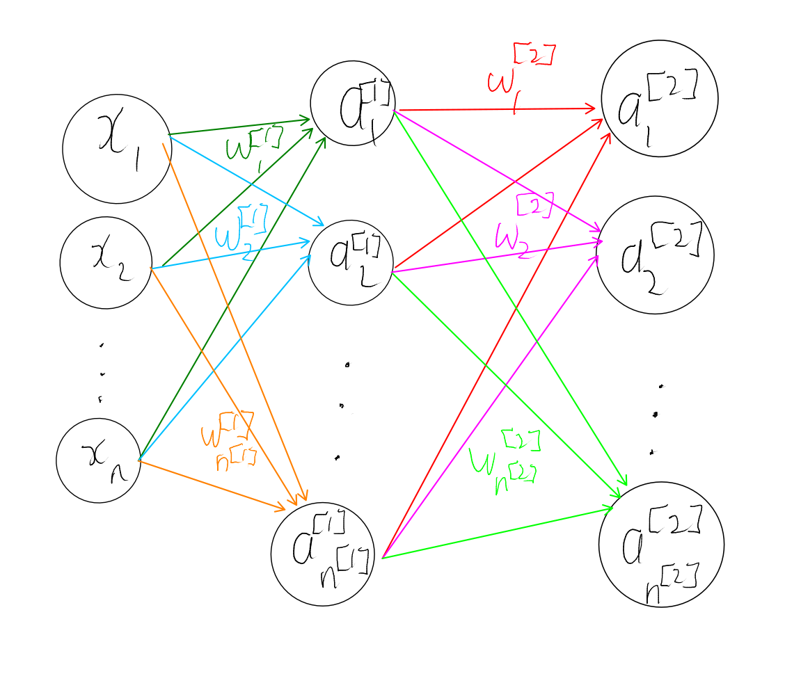
Two layer neural network
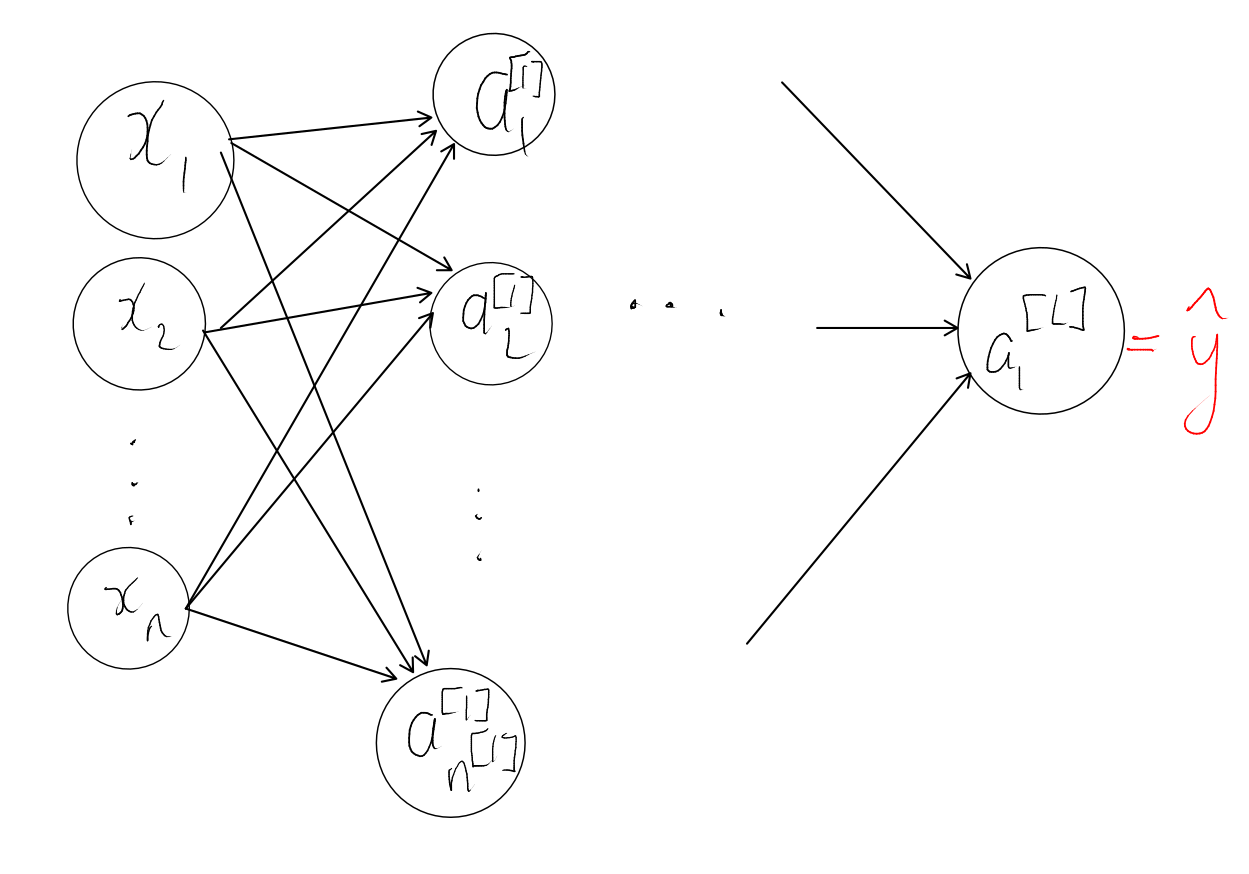
We can keep adding more layers to our network by using the activations of the last layer as inputs to the next layer. However, at the end of the day we want to be predicting a single real value $y\in\mathbb R$. Hence for the last layer we have just a single node, and the value of that node is the model’s prediction.
Also, for the last layer we have to pay a bit more attention to the activation function; for example, if the prediction $\hat y$ should lie in $[0,1]$ then we should apply a sigmoid activation function. However if instead the predicted output can be any real number, then an activation function like sigmoid should not be applied as that would restrict the predicted output to always lie in $[0,1]$.
Vectorization
And that’s all a neural network is! Before we proceed any further, we will vectorize our setup, like we did for linear regression. Recall that we have $m$ training examples pairs $\{(x^{(i)},y^{(i)})\}_{i=1}^m$ for $x_i\in\mathbb R^n,y_i\in\mathbb R$. Later on, we’re going to have to compute $\hat y^{(i)}$ for all $i$ i.e. we need to compute the model’s prediction on each of the training examples $x^{(i)}$. We can do this one by one as per the procedure described above, but it would be better if we could compute all of them in one go.
To accomplish this, arrange the $x^{(i)}$ as rows of a matrix $X$ as we did for linear regression, and similarly arrange the $y^{(i)}$ as rows of a matrix $Y$. Explicitly,
\[X=\begin{bmatrix} \rule[.5ex]{2.5ex}{0.5pt}{x^{(1)}}^T\rule[.5ex]{2.5ex}{0.5pt}\\ \vdots\\ \rule[.5ex]{2.5ex}{0.5pt}{x^{(m)}}^T\rule[.5ex]{2.5ex}{0.5pt}\\ \end{bmatrix}.\]and
\[Y=\begin{bmatrix} y^{(1)}\\ \vdots\\ y^{(m)} \end{bmatrix}.\]Now, we arrange the weights of the first layer as columns of a matrix $W^{[1]}$ i.e.
\[W^{[1]}=\begin{bmatrix} {\rule[-1ex]{0.5pt}{2.5ex}}&&{\rule[-1ex]{0.5pt}{2.5ex}}\\ w_1^{[1]}&\cdots&w_{n^{[1]}}^{[1]}\\ {\rule[-1ex]{0.5pt}{2.5ex}}&&{\rule[-1ex]{0.5pt}{2.5ex}} \end{bmatrix}.\]Matrix multiply $X$ and $W^{[1]}$ to get a matrix
\[Z^{[1]}:=X\cdot W^{[1]}.\]What’s really neat about this is that because of how matrix multiplication works, we actually have
\[Z^{[1]}=\begin{bmatrix} \rule[.5ex]{2.5ex}{0.5pt}{z^{(1)[1]}}^T\rule[.5ex]{2.5ex}{0.5pt}\\ \vdots\\ \rule[.5ex]{2.5ex}{0.5pt}{z^{(m)[1]}}^T\rule[.5ex]{2.5ex}{0.5pt}\\ \end{bmatrix}\]i.e. the $i$th row of $Z^{[1]}$ give us the $z$ values in the first layer of training example $i$.
If we then apply the activation function $g^{[1]}$ elementwise to each component of $Z^{[1]}$ we get a matrix
\[A^{[1]}:=g^{[1]}( Z^{[1]})=\begin{bmatrix} \rule[.5ex]{2.5ex}{0.5pt}{a^{(1)[1]}}^T\rule[.5ex]{2.5ex}{0.5pt}\\ \vdots\\ \rule[.5ex]{2.5ex}{0.5pt}{a^{(m)[1]}}^T\rule[.5ex]{2.5ex}{0.5pt}\\ \end{bmatrix}\]and similar to before, the $i$th row of $A^{[1]}$ gives us the activation values in the first layer of training example $i$.
We can do this process for all layers so that in general, at layer $\ell$ we have
\[\begin{align*} Z^{[\ell]}&:=A^{[\ell-1]}\cdot W^{[\ell]}=\begin{bmatrix} \rule[.5ex]{2.5ex}{0.5pt}{z^{(1)[\ell]}}^T\rule[.5ex]{2.5ex}{0.5pt}\\ \vdots\\ \rule[.5ex]{2.5ex}{0.5pt}{z^{(m)[\ell]}}^T\rule[.5ex]{2.5ex}{0.5pt}\\ \end{bmatrix}\\ A^{[\ell]}&:=g^{[\ell]}( Z^{[\ell]})=\begin{bmatrix} \rule[.5ex]{2.5ex}{0.5pt}{a^{(1)[\ell]}}^T\rule[.5ex]{2.5ex}{0.5pt}\\ \vdots\\ \rule[.5ex]{2.5ex}{0.5pt}{a^{(m)[\ell]}}^T\rule[.5ex]{2.5ex}{0.5pt}\\ \end{bmatrix} \end{align*}.\]For the last layer $L$ the activation values $A^{[L]}$ are the model’s predicted values, which are conveniently laid out in the same shape as $Y$ (the $i$th row contains the predicted/actual value in $A^{[L]}$/$Y$). We will see shortly that, like linear regression, we want to minimize the mean squared error between the predicted and actual values over all the training examples. This error is given by
\[\frac 1m\sum_{i=1}^m(\hat y ^{(i)}-y^{(i)})^2\]which, using our vectorized form, we can write as
\[\frac 1m \Vert A^{[L]}-Y\Vert_F^2\]where $\Vert\cdot\Vert_F$ denotes Frobenius norm (in this case this is the exact same as the $L_2$ norm but it will be helpful to think of vectors as matrices where possible).
Gradient descent
With that out of the way, we now move on to the key issue of neural networks: figuring out what we should set the various weights $W^{[1]},\cdots, W^{[L]}$ to. As alluded to earlier, in our setup for linear regression we picked the weights $w$ so as to minimize the mean squared error between the predicted and actual value over all the training examples
\[f(w)=\frac 1m\sum_{i=1}^m(\hat y ^{(i)}-y^{(i)})^2\]where $\hat y^{(i)}=x^T\cdot w$ denotes the predicted value by the linear regression model and is dependent on $w$, and $y^{(i)}$ denotes the true value. In other words our solution was
\[w^*=\arg\min_wf(w)\]which we were able to compute explicitly by finding the critical points of $f$.
In our setup with neural networks we again want to minimze the mean squared error between the predicted and actual values acros all the training examples
\[f(W)=\frac 1m\sum_{i=1}^m(\hat y ^{(i)}-y^{(i)})^2\]where $\hat y^{(i)}$ denotes the predicted value using our neural network and is dependent on the weights $W:=W^{[1]},\cdots, W^{[L]}$. This time around, however, we are not able to explicitly solve for
\[W^*=\arg\min_wf(W)\]by finding the critical points of $f$ like we did before. Instead, the trick is to approximate $W^*$ by using gradient descent. To do this we need to compute the partial derivatives of $f$ with respect to all the weights. This means that for the matrix $W^{[\ell]}$ at each layer $\ell$ we need to compute the partial derivative of $f$ with respect to each of the components in $W^{[\ell]}$ i.e. we need to compute
\[\frac{\partial f}{\partial W^{[\ell]}_{i,j}}\]for all $i,j,\ell$. This can be done in principal, but to make our lives easier, we will try to take the partial derivative with respect to all the components in $W^{[\ell]}$ in one go. Specifically, let $\frac{\partial f}{\partial W^{[\ell]}}$ denote the matrix containing the partial derivatives with respect to each component of $W^{[\ell]}$ (so that the $i,j$th entry of $\frac{\partial f}{\partial W^{[\ell]}}$ is $\frac{\partial f}{\partial W^{[\ell]}_{i,j}}$), and analogously for $\frac{\partial f}{\partial Z^{[\ell]}},\frac{\partial f}{\partial A^{[\ell]}}$, etc. We would like to compute these quantities using only operations between matrices.
Matrix calculus
Our function $f$ is essentially comprised of a series of matrix-to-matrix operations (e.g. matrix multiplication, or applying an elementwise function to a matrix), followed by a matrix-to-scalar function at the end (i.e. computing the Frobenius norm of a matrix).
We will abstract this as follows: let $G$ be an arbitrary matrix-to-matrix function which takes input $X$, and $f$ be an arbitrary matrix-to-scalar function that takes as input $G$ i.e. we have $f(G(X))$ which is matrix-to-scalar.
Our goal is to find a set of rules for computing \(\frac{df}{dX}\) in terms of the matrix $\frac{df}{dG}$ and the function $G$.
Matrix-to-matrix derivatives
To do this, we first let $f$ be arbitrary and fix $G$. This is best explained by example. Below, $G:\mathbb R^{m\times n}\to\mathbb R^{m\times p}$ is the matrix-to-matrix function that takes its input $X$ and right-multiplies it by a constant matrix $W$ so that $G:X\mapsto X\cdot W$. For this particular $G$, we can calculate $\frac{df}{dX}$ as follows.
Right Matrix multiplication
\[\begin{align*} \frac{df}{dX_{i,j}}&=\sum_{k,\ell}\frac{df}{dG_{k,\ell}}\cdot\frac{dG_{k,\ell}}{dX_{i,j}}\tag{multivariable chain rule}\\ &=\sum_{k,\ell}\frac{df}{dG_{k,\ell}}\cdot\frac{d}{dX_{i,j}}(X_{k,1}W_{1,\ell}+X_{k,2}W_{2,\ell}+\cdots+X_{k,n}W_{n,\ell})\\ &=\sum_{k,\ell}\frac{df}{dG_{k,\ell}}\cdot 1_{k=i}\frac{d}{dX_{i,j}}(X_{k,j}W_{j,\ell})\\ &=\sum_\ell \frac{df}{dG_{i,\ell}}\cdot \frac{d}{dX_{i,j}}(X_{i,j}W_{j,\ell})\\ &=\sum_\ell \frac{df}{dG_{i,\ell}}\cdot W_{j,\ell}\\ &=\sum_\ell \frac{df}{dG_{i,\ell}}\cdot W_{\ell,j}^T\\ \implies \frac{df}{dX}&=\frac{df}{dG}\cdot W^T. \end{align*}\]This is essentially a sort of “chain rule”. We’ve written the derivative $\frac{df}{dX}$ in terms of $\frac{df}{dG}$ and $W$ (which comes from the function $G$). In a proper chain rule, we’d expect to see $\frac{dG}{dX}$ appearing somewhere; the right multiplication of $\frac{df}{dG}$ by $W^T$ takes on this role. It is not immediately clear how to define $\frac{dG}{dX}$ since $G$ is matrix-to-matrix and so $\frac{dG}{dX}$ would have to be 4 dimensional; hence I find it easier to write it in the form I have as above.
Left multiplication by matrix
Using a similar line of reasoning, one can show (exercise to the reader) that if
\[\begin{align*} G:X\mapsto W\cdot X\\ G:\mathbb R^{m\times n}\to\mathbb R^{p\times n} \end{align*}\]where $W\in\mathbb R^{p\times m}$ is a constant, then
\[\frac{df}{dX}=W^T\cdot\frac{df}{dG}.\]Notice here that our function $G$ is different; consequently the role of $\frac{dG}{dX}$ is now taken up by left-multiplying $\frac{df}{dG}$ by $W^T$.
Elementwise function application
Here’s a different example that involves applying a scalar-to-scalar function $g:\mathbb R\to\mathbb R$ elementwise to each entry of a matrix.
Let
\[\begin{align*} G:X\mapsto g(X)\\ g:\mathbb R\to\mathbb R,G:\mathbb R^{m\times n}\to\mathbb R^{m\times n}. \end{align*}\]Then
\[\begin{align*} \frac{df}{dX_{i,j}}&=\sum_{k,\ell}\frac{df}{dG_{k,\ell}}\cdot\frac{dG_{k,\ell}}{dX_{i,j}}\tag{multivariable chain rule}\\ &=\sum_{k,\ell}\frac{df}{dG_{k,\ell}}\cdot\frac{d}{dX_{i,j}}g(X_{k,\ell})\\ &=\sum_{k,\ell}\frac{df}{dG_{k,\ell}}\cdot 1_{k=i,\ell=j}\frac{d}{dX_{i,j}}g(X_{k,\ell})\\ &=\frac{df}{dG_{i,j}}\cdot\frac{d}{dX_{i,j}}g(X_{i,j})\\ &=\frac{df}{dG_{i,j}}\cdot g'(X_{i,j})\\ \implies\frac{df}{dX}&=\frac{df}{dG}\odot (g' (X)). \end{align*}\]where $\odot$ denotes the elementwise (Hadamard) product between two matrices. I want to point out again that now the role of $\frac{dG}{dX}$ is to elementwise multiply $\frac{df}{dG}$ by $g’(X)$.
Matrix addition
Here’s one final (and simple) example that involves adding a constant matrix.
Let
\[\begin{align*} G:X\mapsto X+C\\ G:\mathbb R^{m\times n}\to\mathbb R^{m\times n} \end{align*}\]where $C\in\mathbb R^{m\times n}$ is a constant. Then
\[\begin{align*} \frac{df}{dX_{i,j}}&=\sum_{k,\ell}\frac{df}{dG_{k,\ell}}\cdot\frac{dG_{k,\ell}}{dX_{i,j}}\tag{multivariate chain rule}\\ &=\sum_{k,\ell}\frac{df}{dG_{k,\ell}}\cdot\frac{d}{dX_{i,j}}(X_{k,\ell}+C_{k,\ell})\\ &=\sum_{k,\ell}\frac{df}{dG_{k,\ell}}\cdot 1_{k=i,\ell=j}\frac{d}{dX_{i,j}}(X_{k,\ell}+C_{k,\ell})\\ &=\frac{df}{dG_{i,j}}\cdot\frac{d}{dX_{i,j}}(X_{i,j}+C_{i,j})\\ &=\frac{df}{dG_{i,j}}\\ \implies \frac{df}{dX}&=\frac{df}{dG}. \end{align*}\]This is just a fancy way of saying that adding constants does not change the derivative.
Matrix-to-scalar derivatives
So far we have written $\frac{df}{dX}$ in terms of $\frac{df}{dG}$. I now explain how to compute $\frac{df}{dG}$. We now let $G$ be arbitrary and fix $f$. In the below example $f$ computes the squared Frobenius norm.
Squared Frobenius norm
Let
\[\begin{align*} f:G\mapsto \Vert G\Vert_F^2\\ f:\mathbb R^{m\times n}\to\mathbb R \end{align*}\]Then
\[\begin{align*} \frac{df}{dG_{i,j}}&=\frac{d}{dG_{i,j}}\sum_{k,\ell}G_{k,\ell}^2\\ &=\frac{d}{dG_{i,j}}G_{i,j}^2\\ &=2G_{i,j}\\ \implies \frac{df}{dG}&=2G. \end{align*}\]Derivative calculations
We now have all the pieces available to compute the derivatives in our neural network.
Derivative with respect to $A^{[L]}$
Recall that if we have the model’s predictions $A^{[L]}$ we define the loss to be
\(f(A^{[L]})=\frac 1m\Vert A^{[L]}-Y\Vert_F^2\) Let’s calculate
\[\frac{df}{dA^{[L]}}.\]We have
\[\begin{align*} \frac{df}{dA^{[L]}}&=\frac{d(\frac 1m\Vert A^{[L]}-Y\Vert_F^2)}{dA^{[L]}}\\ &=\frac 1m\frac{d(\Vert A^{[L]}-Y\Vert_F^2)}{dA^{[L]}}\\ &=\frac 1m\frac{d(\Vert A^{[L]}-Y\Vert_F^2)}{d(A^{[L]}-Y)}\\ &=\frac 1m\cdot 2(A^{[L]}-Y).\\ \end{align*}\]To get to the second last line we have used our matrix calculus framework with the matrix-to-matrix function $G:A^{[L]}\mapsto A^{[L]}-Y$. To get to the last line, we have again used our matrix calculus framework, this time with the matrix-to-scalar function $f:A^{[L]}-Y\mapsto \Vert A^{[L]}-Y\Vert_F^2$.
Derivative with respect to $Z^{[L]}$
Recall that $A^{[L]}=g^{[L]}(Z^{[L]})$ where $g^{[L]}$ is the activation function of the last layer. We can calculate
\[\frac{df}{dZ^{[L]}}\]using our matrix calculus framework since
\[\begin{align*} \frac{df}{dZ^{[L]}}&=\frac{df}{dA^{[L]}}\odot {g^{[L]}}'(Z^{[L]})\\ &=\frac 2m (A^{[L]}-Y)\odot ({g^{[L]}}'(Z^{[L]})). \end{align*}\]The first equality is due to the matrix calculus framework with matrix-to-matrix function $G:Z^{[L]}\mapsto g^{[L]}(Z^{[L]})$ and the second equality is due to substituting our computation for $\frac{df}{dA^{[L]}}$ that we just did above.
Derivative with respect to $W^{[L]}$
We can now calculate
\[\frac{df}{dW^{[L]}}\]which is one of the terms that we need to calculate for gradient descent. Recalling that $Z^{[L]}=A^{[L-1]}\cdot W^{[L]}$, we have
\[\begin{align*} \frac{df}{dW^{[L]}}&={A^{[L-1]}}^T\cdot\frac{df}{dZ^{[L]}}\\ &=\frac 2m {A^{[L-1]}}^T\cdot (A^{[L]}-Y)\odot ({g^{[L]}}'(Z^{[L]})). \end{align*}\]The first equality is due to the matrix calculus framework with matrix-to-matrix function $G:W^{[L]}\mapsto A^{[L-1]}\cdot W^{[L]}$ and the second equality is due to substituting the result above.
Derivatives in an arbitrary layer
It’s now pretty easy to calculate the derivatives in any arbitrary layer. First, let’s calculate $\frac{df}{dA^{[\ell]}}$ for a non-final layer $\ell=1,2,\cdots,L-1$. Notice that $A^{[\ell]}$ is used as the “input” for the next layer $\ell+1$ i.e.
\[Z^{[\ell+1]}=A^{[\ell]}\cdot W^{[\ell+1]}.\]Our matrix calculus framework then tells us
\[\frac{df}{dA^{[\ell]}}=\frac{df}{dZ^{[\ell+1]}}\cdot {W^{[\ell+1]}}^T\]We can calculate the derivatives with respect to $Z^{[\ell]}$ and $W^{[\ell]}$ in the exact same way that we calculated the derivatives for $Z^{[L]}$ and $W^{[L]}$ respectively (check yourself), so we get
\[\frac{df}{dZ^{[\ell]}}=\frac{df}{dA^{[\ell]}}\odot (g'( Z^{[\ell]}))\\ \frac{df}{dW^{[\ell]}}={A^{[\ell-1]}}^T\cdot\frac{df}{dZ^{[\ell]}}\]Derivative summary
To summarise, our matrix calculus framework allowed us to compute the derivatives of the loss function with respect to any matrix quantity in our neural network. Explicitly, we have
\[\begin{align*} \frac{df}{dA^{[L]}}=\frac 1m\cdot 2(A^{[L]}-Y)\\ \frac{df}{dA^{[\ell]}}=\frac{df}{dZ^{[\ell+1]}}\cdot {W^{[\ell+1]}}^T,&\qquad \ell =1,2,\cdots,L-1\\ \frac{df}{dZ^{[\ell]}}=\frac{df}{dA^{[\ell]}}\odot (g'( Z^{[\ell]})),&\qquad \ell=1,2,\cdots,L\\ \frac{df}{dW^{[\ell]}}={A^{[\ell-1]}}^T\cdot\frac{df}{dZ^{[\ell]}},&\qquad\ell=1,2,\cdots,L \end{align*}\]Final notes
Note that although we only needed to calculate $\frac{df}{dW^{[\ell]}}$, we also calculated $\frac{df}{dA^{[\ell]}}$ and $\frac{df}{dZ^{[\ell]}}$ as they are required in intermediate calculations.
Now that we’ve calculated $\frac{df}{dW^{[\ell]}}$, we can apply gradient descent to approximate $W^*$, the optimal set of weights that result in the lowest MSE across all the training examples. To do this, typically all the weights are initialized randomly, and the weights are updated as
\[W^{[\ell]}\leftarrow W^{[\ell]}-\alpha \cdot \frac{df}{dW^{[\ell]}}\]where $\alpha>0$ is the learning rate. In practice, variations of the traditional gradient descent update rule are used instead (e.g. Adam), though we will not discuss about them in depth here.